Fits generalized boosted regression models. For technical details, see the
vignette: utils::browseVignettes("gbm").
Usage
gbm(
  formula = formula(data),
  distribution = "bernoulli",
  data = list(),
  weights,
  var.monotone = NULL,
  n.trees = 100,
  interaction.depth = 1,
  n.minobsinnode = 10,
  shrinkage = 0.1,
  bag.fraction = 0.5,
  train.fraction = 1,
  cv.folds = 0,
  keep.data = TRUE,
  verbose = FALSE,
  class.stratify.cv = NULL,
  n.cores = NULL
)
Arguments
- formula
A symbolic description of the model to be fit. The formula may include an offset term (e.g. y~offset(n)+x). If
keep.data = FALSEin the initial call togbmthen it is the user's responsibility to resupply the offset togbm.more.- distribution
Either a character string specifying the name of the distribution to use or a list with a component
namespecifying the distribution and any additional parameters needed. If not specified,gbmwill try to guess: if the response has only 2 unique values, bernoulli is assumed; otherwise, if the response is a factor, multinomial is assumed; otherwise, if the response has class"Surv", coxph is assumed; otherwise, gaussian is assumed.Currently available options are
"gaussian"(squared error),"laplace"(absolute loss),"tdist"(t-distribution loss),"bernoulli"(logistic regression for 0-1 outcomes),"huberized"(huberized hinge loss for 0-1 outcomes),"adaboost"(the AdaBoost exponential loss for 0-1 outcomes),"poisson"(count outcomes),"coxph"(right censored observations),"quantile", or"pairwise"(ranking measure using the LambdaMart algorithm).If quantile regression is specified,
distributionmust be a list of the formlist(name = "quantile", alpha = 0.25)wherealphais the quantile to estimate.If
"tdist"is specified, the default degrees of freedom is 4 and this can be controlled by specifyingdistribution = list(name = "tdist", df = DF)whereDFis your chosen degrees of freedom.If "pairwise" regression is specified,
distributionmust be a list of the formlist(name="pairwise",group=...,metric=...,max.rank=...)(metricandmax.rankare optional, see below).groupis a character vector with the column names ofdatathat jointly indicate the group an instance belongs to (typically a query in Information Retrieval applications). For training, only pairs of instances from the same group and with different target labels can be considered.metricis the IR measure to use, one of- list("conc")
Fraction of concordant pairs; for binary labels, this is equivalent to the Area under the ROC Curve
- :
Fraction of concordant pairs; for binary labels, this is equivalent to the Area under the ROC Curve
- list("mrr")
Mean reciprocal rank of the highest-ranked positive instance
- :
Mean reciprocal rank of the highest-ranked positive instance
- list("map")
Mean average precision, a generalization of
mrrto multiple positive instances- :
Mean average precision, a generalization of
mrrto multiple positive instances- list("ndcg:")
Normalized discounted cumulative gain. The score is the weighted sum (DCG) of the user-supplied target values, weighted by log(rank+1), and normalized to the maximum achievable value. This is the default if the user did not specify a metric.
ndcgandconcallow arbitrary target values, while binary targets {0,1} are expected formapandmrr. Forndcgandmrr, a cut-off can be chosen using a positive integer parametermax.rank. If left unspecified, all ranks are taken into account.Note that splitting of instances into training and validation sets follows group boundaries and therefore only approximates the specified
train.fractionratio (the same applies to cross-validation folds). Internally, queries are randomly shuffled before training, to avoid bias.Weights can be used in conjunction with pairwise metrics, however it is assumed that they are constant for instances from the same group.
For details and background on the algorithm, see e.g. Burges (2010).
- data
an optional data frame containing the variables in the model. By default the variables are taken from
environment(formula), typically the environment from whichgbmis called. Ifkeep.data=TRUEin the initial call togbmthengbmstores a copy with the object. Ifkeep.data=FALSEthen subsequent calls togbm.moremust resupply the same dataset. It becomes the user's responsibility to resupply the same data at this point.- weights
an optional vector of weights to be used in the fitting process. Must be positive but do not need to be normalized. If
keep.data=FALSEin the initial call togbmthen it is the user's responsibility to resupply the weights togbm.more.- var.monotone
an optional vector, the same length as the number of predictors, indicating which variables have a monotone increasing (+1), decreasing (-1), or arbitrary (0) relationship with the outcome.
- n.trees
Integer specifying the total number of trees to fit. This is equivalent to the number of iterations and the number of basis functions in the additive expansion. Default is 100.
- interaction.depth
Integer specifying the maximum depth of each tree (i.e., the highest level of variable interactions allowed). A value of 1 implies an additive model, a value of 2 implies a model with up to 2-way interactions, etc. Default is 1.
- n.minobsinnode
Integer specifying the minimum number of observations in the terminal nodes of the trees. Note that this is the actual number of observations, not the total weight.
- shrinkage
a shrinkage parameter applied to each tree in the expansion. Also known as the learning rate or step-size reduction; 0.001 to 0.1 usually work, but a smaller learning rate typically requires more trees. Default is 0.1.
- bag.fraction
the fraction of the training set observations randomly selected to propose the next tree in the expansion. This introduces randomnesses into the model fit. If
bag.fraction< 1 then running the same model twice will result in similar but different fits.gbmuses the R random number generator soset.seedcan ensure that the model can be reconstructed. Preferably, the user can save the returnedgbm.objectusingsave. Default is 0.5.- train.fraction
The first
train.fraction * nrows(data)observations are used to fit thegbmand the remainder are used for computing out-of-sample estimates of the loss function.- cv.folds
Number of cross-validation folds to perform. If
cv.folds>1 thengbm, in addition to the usual fit, will perform a cross-validation, calculate an estimate of generalization error returned incv.error. Ifcv.folds=1,gbmwarns and proceeds without cross-validation.- keep.data
a logical variable indicating whether to keep the data and an index of the data stored with the object. Keeping the data and index makes subsequent calls to
gbm.morefaster at the cost of storing an extra copy of the dataset.- verbose
Logical indicating whether or not to print out progress and performance indicators (
TRUE). If this option is left unspecified forgbm.more, then it usesverbosefromobject. Default isFALSE.- class.stratify.cv
Logical indicating whether or not the cross-validation should be stratified by class. Defaults to
TRUEfordistribution = "multinomial"and is only implemented for"multinomial"and"bernoulli". The purpose of stratifying the cross-validation is to help avoiding situations in which training sets do not contain all classes.- n.cores
The number of CPU cores to use. The cross-validation loop will attempt to send different CV folds off to different cores. If
n.coresis not specified by the user, it is guessed using thedetectCoresfunction in theparallelpackage. Note that the documentation fordetectCoresmakes clear that it is not failsafe and could return a spurious number of available cores.
Value
A gbm.object object.
Details
gbm.fit provides the link between R and the C++ gbm engine.
gbm is a front-end to gbm.fit that uses the familiar R
modeling formulas. However, model.frame is very slow if
there are many predictor variables. For power-users with many variables use
gbm.fit. For general practice gbm is preferable.
This package implements the generalized boosted modeling framework. Boosting is the process of iteratively adding basis functions in a greedy fashion so that each additional basis function further reduces the selected loss function. This implementation closely follows Friedman's Gradient Boosting Machine (Friedman, 2001).
In addition to many of the features documented in the Gradient Boosting
Machine, gbm offers additional features including the out-of-bag
estimator for the optimal number of iterations, the ability to store and
manipulate the resulting gbm object, and a variety of other loss
functions that had not previously had associated boosting algorithms,
including the Cox partial likelihood for censored data, the poisson
likelihood for count outcomes, and a gradient boosting implementation to
minimize the AdaBoost exponential loss function. This gbm package is no
longer under further development. Consider
https://github.com/gbm-developers/gbm3 for the latest version.
References
Y. Freund and R.E. Schapire (1997) “A decision-theoretic generalization of on-line learning and an application to boosting,” Journal of Computer and System Sciences, 55(1):119-139.
G. Ridgeway (1999). “The state of boosting,” Computing Science and Statistics 31:172-181.
J.H. Friedman, T. Hastie, R. Tibshirani (2000). “Additive Logistic Regression: a Statistical View of Boosting,” Annals of Statistics 28(2):337-374.
J.H. Friedman (2001). “Greedy Function Approximation: A Gradient Boosting Machine,” Annals of Statistics 29(5):1189-1232.
J.H. Friedman (2002). “Stochastic Gradient Boosting,” Computational Statistics and Data Analysis 38(4):367-378.
B. Kriegler (2007). Cost-Sensitive Stochastic Gradient Boosting Within a Quantitative Regression Framework. Ph.D. Dissertation. University of California at Los Angeles, Los Angeles, CA, USA. Advisor(s) Richard A. Berk. https://dl.acm.org/doi/book/10.5555/1354603.
C. Burges (2010). “From RankNet to LambdaRank to LambdaMART: An Overview,” Microsoft Research Technical Report MSR-TR-2010-82.
Author
Greg Ridgeway gregridgeway@gmail.com
Quantile regression code developed by Brian Kriegler bk@stat.ucla.edu
t-distribution, and multinomial code developed by Harry Southworth and Daniel Edwards
Pairwise code developed by Stefan Schroedl schroedl@a9.com
Examples
#
# A least squares regression example
#
# Simulate data
set.seed(101) # for reproducibility
N <- 200
X1 <- runif(N)
X2 <- 2 * runif(N)
X3 <- ordered(sample(letters[1:4], N, replace = TRUE), levels = letters[4:1])
X4 <- factor(sample(letters[1:6], N, replace = TRUE))
X5 <- factor(sample(letters[1:3], N, replace = TRUE))
X6 <- 3 * runif(N)
mu <- c(-1, 0, 1, 2)[as.numeric(X3)]
SNR <- 10 # signal-to-noise ratio
Y <- X1 ^ 1.5 + 2 * (X2 ^ 0.5) + mu
sigma <- sqrt(var(Y) / SNR)
Y <- Y + rnorm(N, 0, sigma)
X1[sample(1:N, size = 100)] <- NA # introduce some missing values
X4[sample(1:N, size = 60)] <- NA # introduce some missing values
data <- data.frame(Y, X1, X2, X3, X4, X5, X6)
# Fit a GBM
set.seed(102) # for reproducibility
gbm1 <- gbm(Y ~ ., data = data, var.monotone = c(0, 0, 0, 0, 0, 0),
distribution = "gaussian", n.trees = 50, shrinkage = 0.1,
interaction.depth = 3, bag.fraction = 0.5, train.fraction = 0.5,
n.minobsinnode = 5, cv.folds = 2, keep.data = TRUE,
verbose = FALSE, n.cores = 1)
#> CV: 1
#> CV: 2
# Check performance using the out-of-bag (OOB) error; the OOB error typically
# underestimates the optimal number of iterations
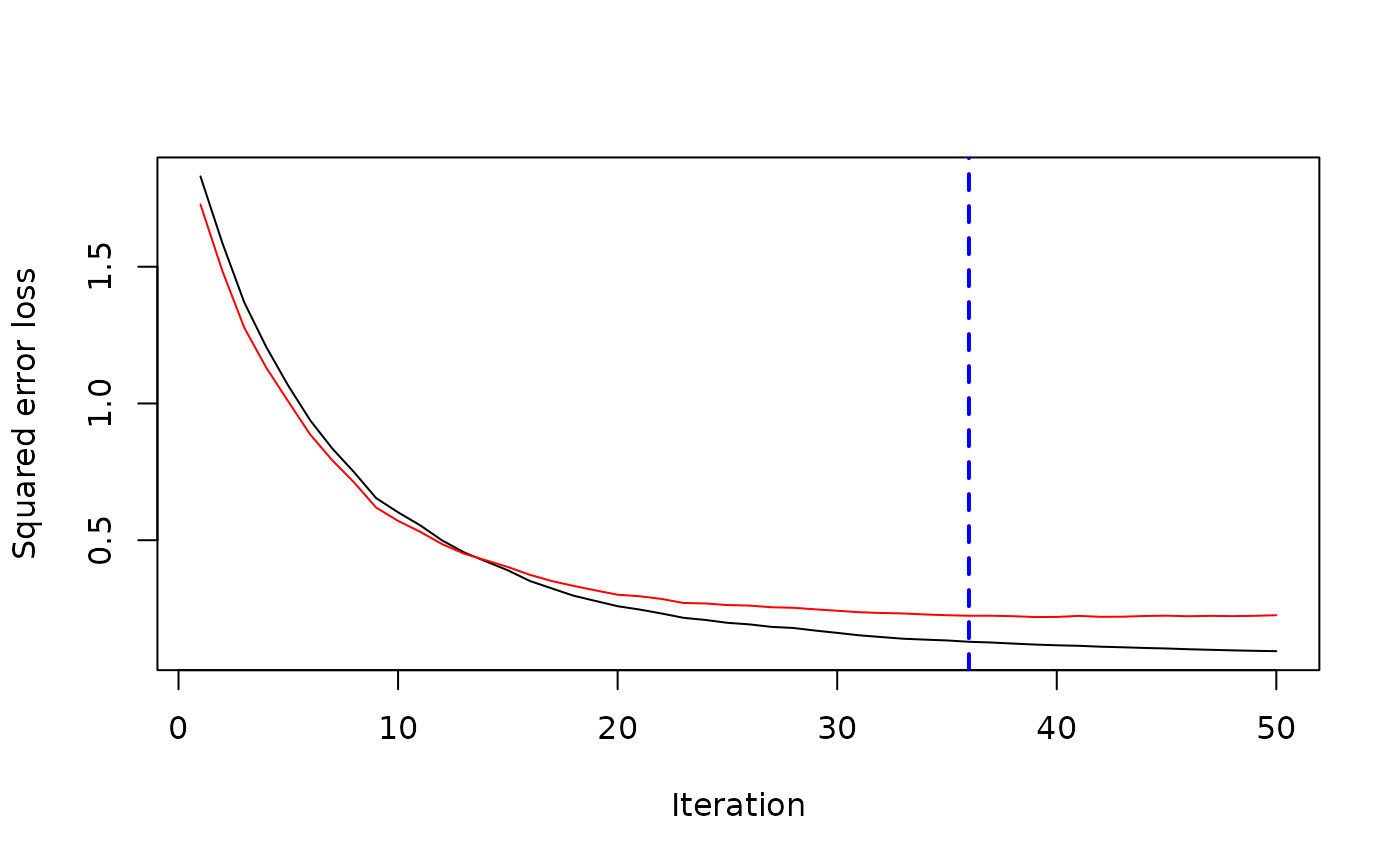
best.iter <- gbm.perf(gbm1, method = "OOB")
#> OOB generally underestimates the optimal number of iterations although predictive performance is reasonably competitive. Using cv_folds>1 when calling gbm usually results in improved predictive performance.
 print(best.iter)
#> [1] 36
#> attr(,"smoother")
#> Call:
#> loess(formula = object$oobag.improve ~ x, enp.target = min(max(4,
#> length(x)/10), 50))
#>
#> Number of Observations: 50
#> Equivalent Number of Parameters: 4.48
#> Residual Standard Error: 0.02081
# Check performance using the 50% heldout test set
best.iter <- gbm.perf(gbm1, method = "test")
print(best.iter)
#> [1] 36
#> attr(,"smoother")
#> Call:
#> loess(formula = object$oobag.improve ~ x, enp.target = min(max(4,
#> length(x)/10), 50))
#>
#> Number of Observations: 50
#> Equivalent Number of Parameters: 4.48
#> Residual Standard Error: 0.02081
# Check performance using the 50% heldout test set
best.iter <- gbm.perf(gbm1, method = "test")
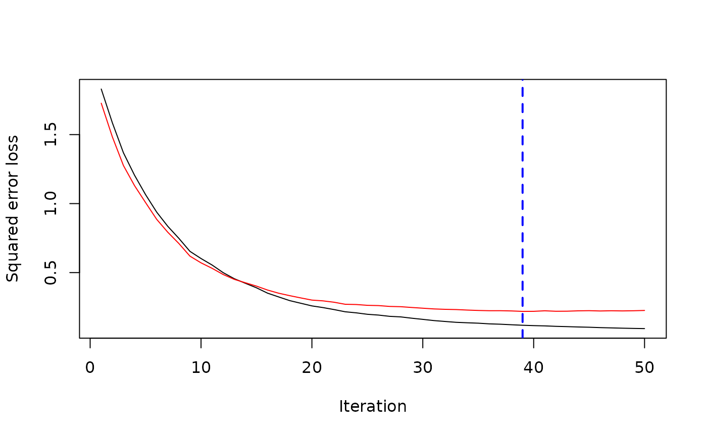 print(best.iter)
#> [1] 39
# Check performance using 2-fold cross-validation
best.iter <- gbm.perf(gbm1, method = "cv")
print(best.iter)
#> [1] 39
# Check performance using 2-fold cross-validation
best.iter <- gbm.perf(gbm1, method = "cv")
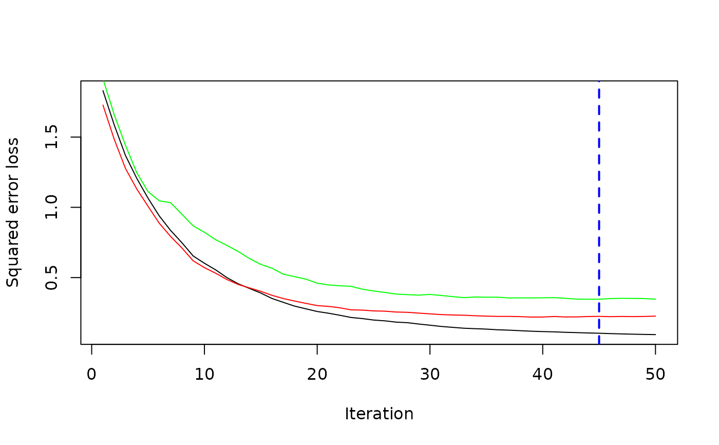 print(best.iter)
#> [1] 45
# Plot relative influence of each variable
par(mfrow = c(1, 2))
summary(gbm1, n.trees = 1) # using first tree
#> var rel.inf
#> X3 X3 92.980497
#> X2 X2 7.019503
#> X1 X1 0.000000
#> X4 X4 0.000000
#> X5 X5 0.000000
#> X6 X6 0.000000
summary(gbm1, n.trees = best.iter) # using estimated best number of trees
print(best.iter)
#> [1] 45
# Plot relative influence of each variable
par(mfrow = c(1, 2))
summary(gbm1, n.trees = 1) # using first tree
#> var rel.inf
#> X3 X3 92.980497
#> X2 X2 7.019503
#> X1 X1 0.000000
#> X4 X4 0.000000
#> X5 X5 0.000000
#> X6 X6 0.000000
summary(gbm1, n.trees = best.iter) # using estimated best number of trees
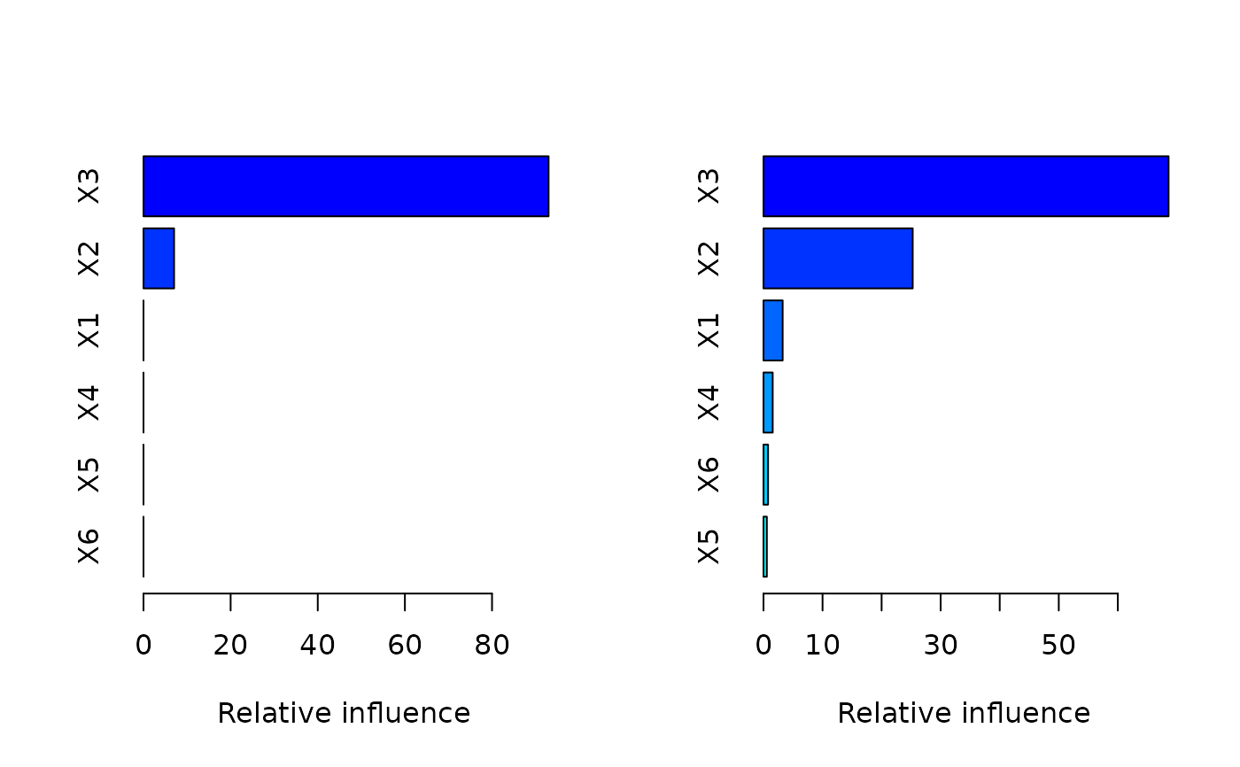 #> var rel.inf
#> X3 X3 68.5940534
#> X2 X2 25.2670646
#> X1 X1 3.2443435
#> X4 X4 1.5579291
#> X6 X6 0.7697113
#> X5 X5 0.5668980
# Compactly print the first and last trees for curiosity
print(pretty.gbm.tree(gbm1, i.tree = 1))
#> SplitVar SplitCodePred LeftNode RightNode MissingNode ErrorReduction Weight
#> 0 2 0.500000000 1 2 9 62.884382 50
#> 1 -1 -0.196847194 -1 -1 -1 0.000000 12
#> 2 2 2.500000000 3 7 8 27.189818 38
#> 3 1 0.636963733 4 5 6 6.800094 29
#> 4 -1 -0.043326682 -1 -1 -1 0.000000 11
#> 5 -1 0.056471781 -1 -1 -1 0.000000 18
#> 6 -1 0.018617191 -1 -1 -1 0.000000 29
#> 7 -1 0.217581278 -1 -1 -1 0.000000 9
#> 8 -1 0.065740265 -1 -1 -1 0.000000 38
#> 9 -1 0.002719275 -1 -1 -1 0.000000 50
#> Prediction
#> 0 0.002719275
#> 1 -0.196847194
#> 2 0.065740265
#> 3 0.018617191
#> 4 -0.043326682
#> 5 0.056471781
#> 6 0.018617191
#> 7 0.217581278
#> 8 0.065740265
#> 9 0.002719275
print(pretty.gbm.tree(gbm1, i.tree = gbm1$n.trees))
#> SplitVar SplitCodePred LeftNode RightNode MissingNode ErrorReduction Weight
#> 0 1 1.652568149 1 8 9 0.7376303 50
#> 1 3 21.000000000 2 3 7 0.4441211 41
#> 2 -1 -0.029987473 -1 -1 -1 0.0000000 8
#> 3 5 1.783450092 4 5 6 0.2890577 20
#> 4 -1 -0.009979236 -1 -1 -1 0.0000000 14
#> 5 -1 0.016254951 -1 -1 -1 0.0000000 6
#> 6 -1 -0.002108980 -1 -1 -1 0.0000000 20
#> 7 -1 -0.010104993 -1 -1 -1 0.0000000 13
#> 8 -1 0.021530848 -1 -1 -1 0.0000000 9
#> 9 -1 -0.004393333 -1 -1 -1 0.0000000 50
#> Prediction
#> 0 -0.004393333
#> 1 -0.010084007
#> 2 -0.029987473
#> 3 -0.002108980
#> 4 -0.009979236
#> 5 0.016254951
#> 6 -0.002108980
#> 7 -0.010104993
#> 8 0.021530848
#> 9 -0.004393333
# Simulate new data
set.seed(103) # for reproducibility
N <- 200
X1 <- runif(N)
X2 <- 2 * runif(N)
X3 <- ordered(sample(letters[1:4], N, replace = TRUE))
X4 <- factor(sample(letters[1:6], N, replace = TRUE))
X5 <- factor(sample(letters[1:3], N, replace = TRUE))
X6 <- 3 * runif(N)
mu <- c(-1, 0, 1, 2)[as.numeric(X3)]
Y <- X1 ^ 1.5 + 2 * (X2 ^ 0.5) + mu + rnorm(N, 0, sigma)
data2 <- data.frame(Y, X1, X2, X3, X4, X5, X6)
# Predict on the new data using the "best" number of trees; by default,
# predictions will be on the link scale
Yhat <- predict(gbm1, newdata = data2, n.trees = best.iter, type = "link")
# least squares error
print(sum((data2$Y - Yhat)^2))
#> [1] 1050.048
# Construct univariate partial dependence plots
plot(gbm1, i.var = 1, n.trees = best.iter)
#> var rel.inf
#> X3 X3 68.5940534
#> X2 X2 25.2670646
#> X1 X1 3.2443435
#> X4 X4 1.5579291
#> X6 X6 0.7697113
#> X5 X5 0.5668980
# Compactly print the first and last trees for curiosity
print(pretty.gbm.tree(gbm1, i.tree = 1))
#> SplitVar SplitCodePred LeftNode RightNode MissingNode ErrorReduction Weight
#> 0 2 0.500000000 1 2 9 62.884382 50
#> 1 -1 -0.196847194 -1 -1 -1 0.000000 12
#> 2 2 2.500000000 3 7 8 27.189818 38
#> 3 1 0.636963733 4 5 6 6.800094 29
#> 4 -1 -0.043326682 -1 -1 -1 0.000000 11
#> 5 -1 0.056471781 -1 -1 -1 0.000000 18
#> 6 -1 0.018617191 -1 -1 -1 0.000000 29
#> 7 -1 0.217581278 -1 -1 -1 0.000000 9
#> 8 -1 0.065740265 -1 -1 -1 0.000000 38
#> 9 -1 0.002719275 -1 -1 -1 0.000000 50
#> Prediction
#> 0 0.002719275
#> 1 -0.196847194
#> 2 0.065740265
#> 3 0.018617191
#> 4 -0.043326682
#> 5 0.056471781
#> 6 0.018617191
#> 7 0.217581278
#> 8 0.065740265
#> 9 0.002719275
print(pretty.gbm.tree(gbm1, i.tree = gbm1$n.trees))
#> SplitVar SplitCodePred LeftNode RightNode MissingNode ErrorReduction Weight
#> 0 1 1.652568149 1 8 9 0.7376303 50
#> 1 3 21.000000000 2 3 7 0.4441211 41
#> 2 -1 -0.029987473 -1 -1 -1 0.0000000 8
#> 3 5 1.783450092 4 5 6 0.2890577 20
#> 4 -1 -0.009979236 -1 -1 -1 0.0000000 14
#> 5 -1 0.016254951 -1 -1 -1 0.0000000 6
#> 6 -1 -0.002108980 -1 -1 -1 0.0000000 20
#> 7 -1 -0.010104993 -1 -1 -1 0.0000000 13
#> 8 -1 0.021530848 -1 -1 -1 0.0000000 9
#> 9 -1 -0.004393333 -1 -1 -1 0.0000000 50
#> Prediction
#> 0 -0.004393333
#> 1 -0.010084007
#> 2 -0.029987473
#> 3 -0.002108980
#> 4 -0.009979236
#> 5 0.016254951
#> 6 -0.002108980
#> 7 -0.010104993
#> 8 0.021530848
#> 9 -0.004393333
# Simulate new data
set.seed(103) # for reproducibility
N <- 200
X1 <- runif(N)
X2 <- 2 * runif(N)
X3 <- ordered(sample(letters[1:4], N, replace = TRUE))
X4 <- factor(sample(letters[1:6], N, replace = TRUE))
X5 <- factor(sample(letters[1:3], N, replace = TRUE))
X6 <- 3 * runif(N)
mu <- c(-1, 0, 1, 2)[as.numeric(X3)]
Y <- X1 ^ 1.5 + 2 * (X2 ^ 0.5) + mu + rnorm(N, 0, sigma)
data2 <- data.frame(Y, X1, X2, X3, X4, X5, X6)
# Predict on the new data using the "best" number of trees; by default,
# predictions will be on the link scale
Yhat <- predict(gbm1, newdata = data2, n.trees = best.iter, type = "link")
# least squares error
print(sum((data2$Y - Yhat)^2))
#> [1] 1050.048
# Construct univariate partial dependence plots
plot(gbm1, i.var = 1, n.trees = best.iter)
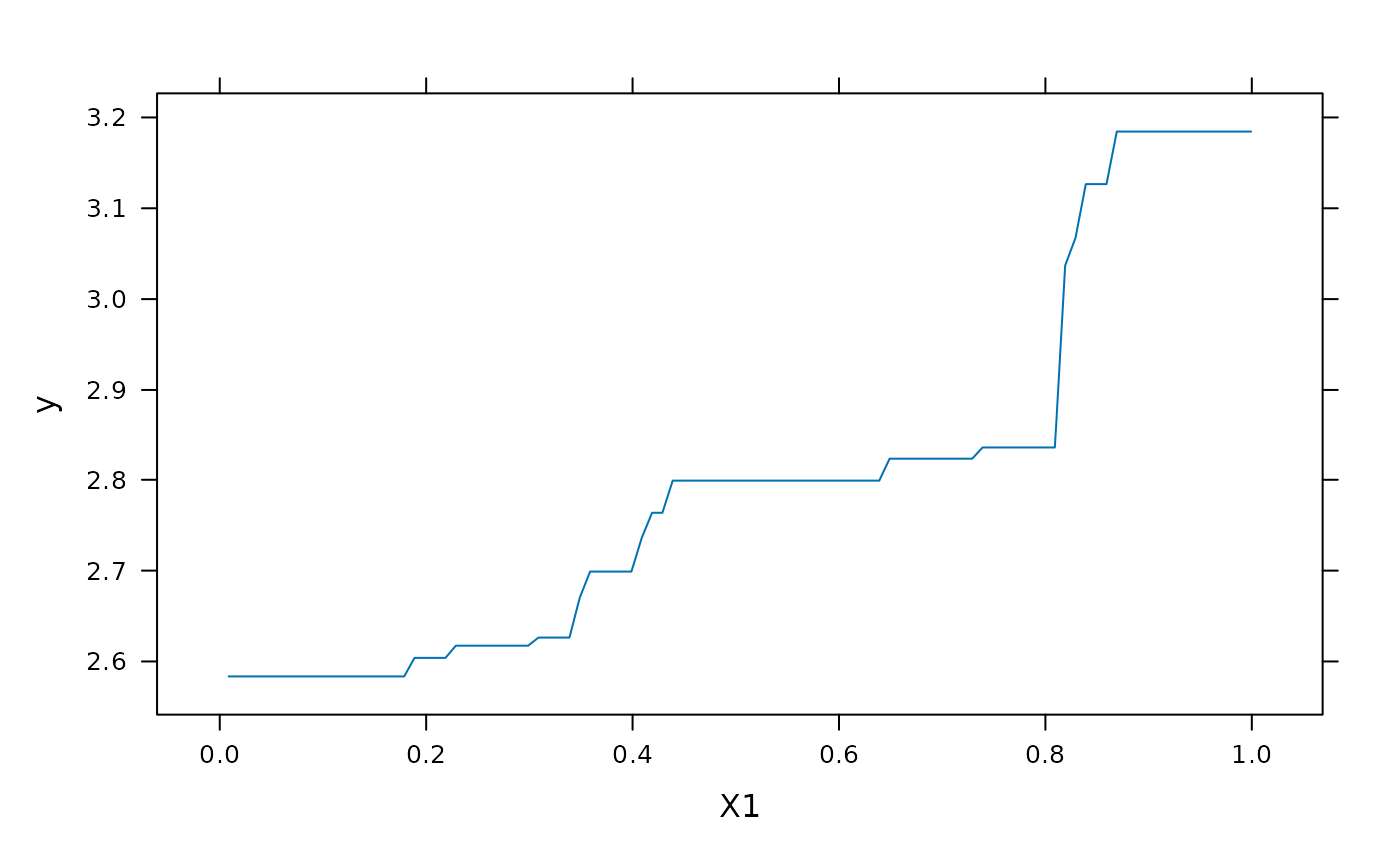 plot(gbm1, i.var = 2, n.trees = best.iter)
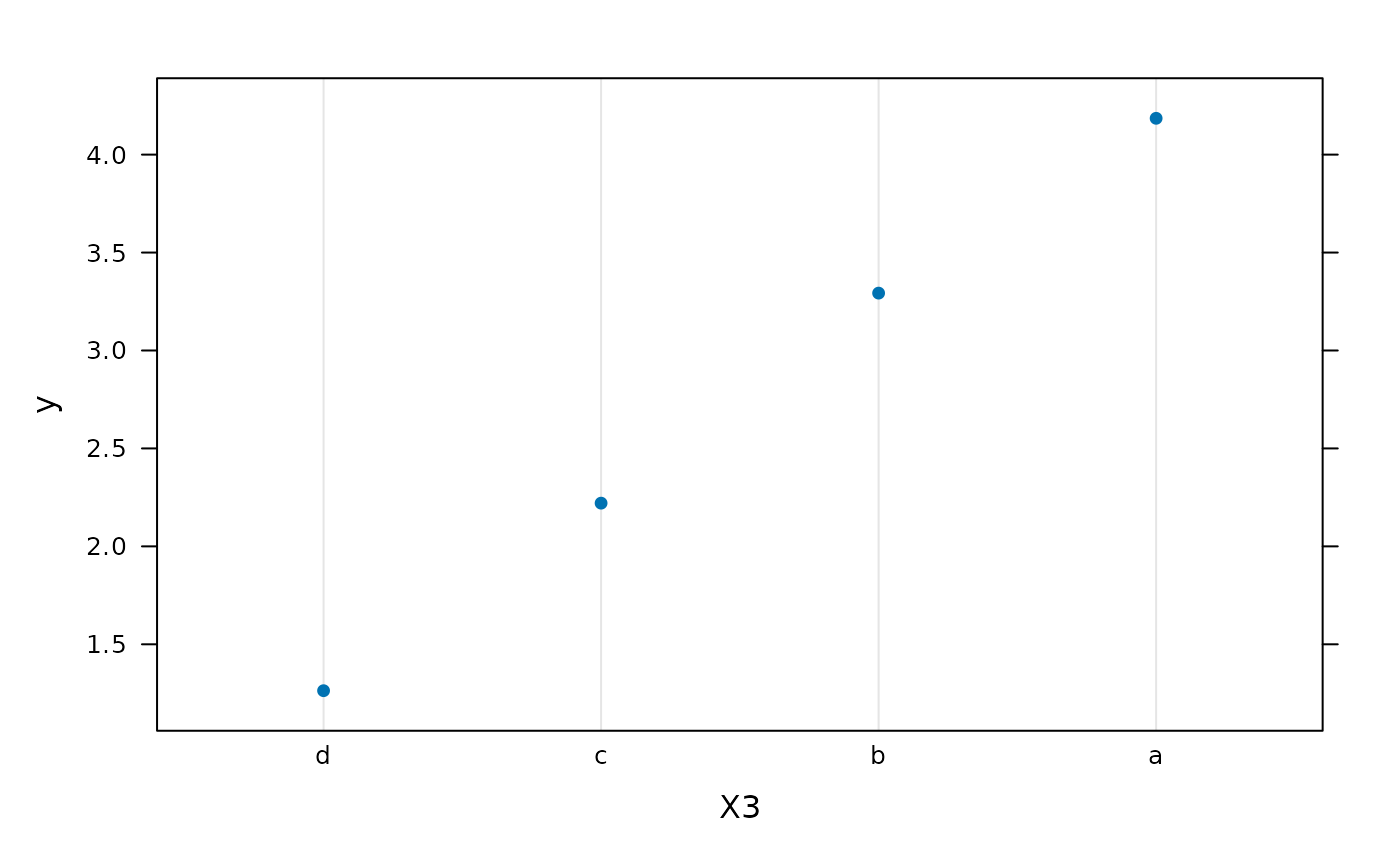
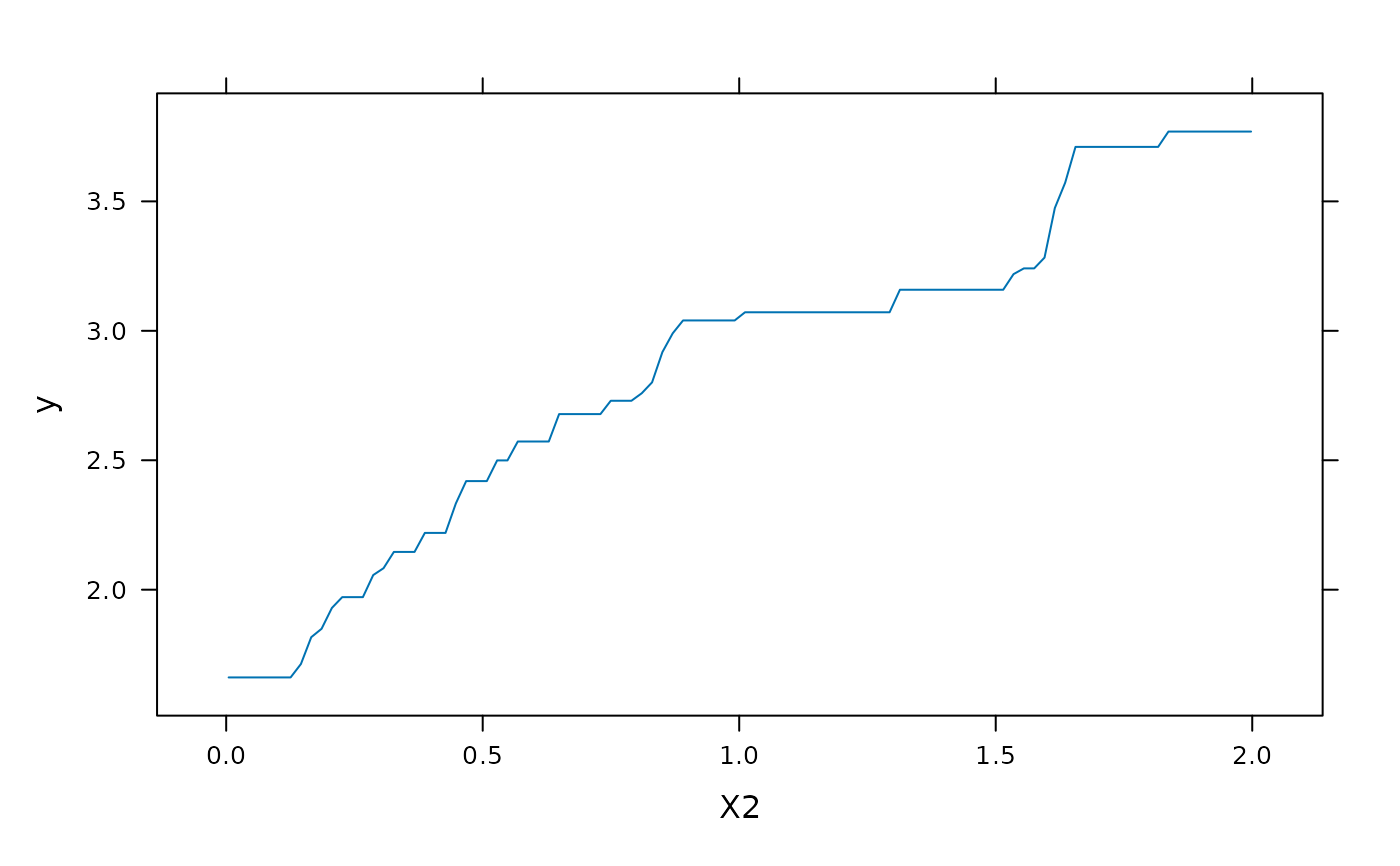 plot(gbm1, i.var = "X3", n.trees = best.iter) # can use index or name
 # Construct bivariate partial dependence plots
plot(gbm1, i.var = 1:2, n.trees = best.iter)
# Construct bivariate partial dependence plots
plot(gbm1, i.var = 1:2, n.trees = best.iter)
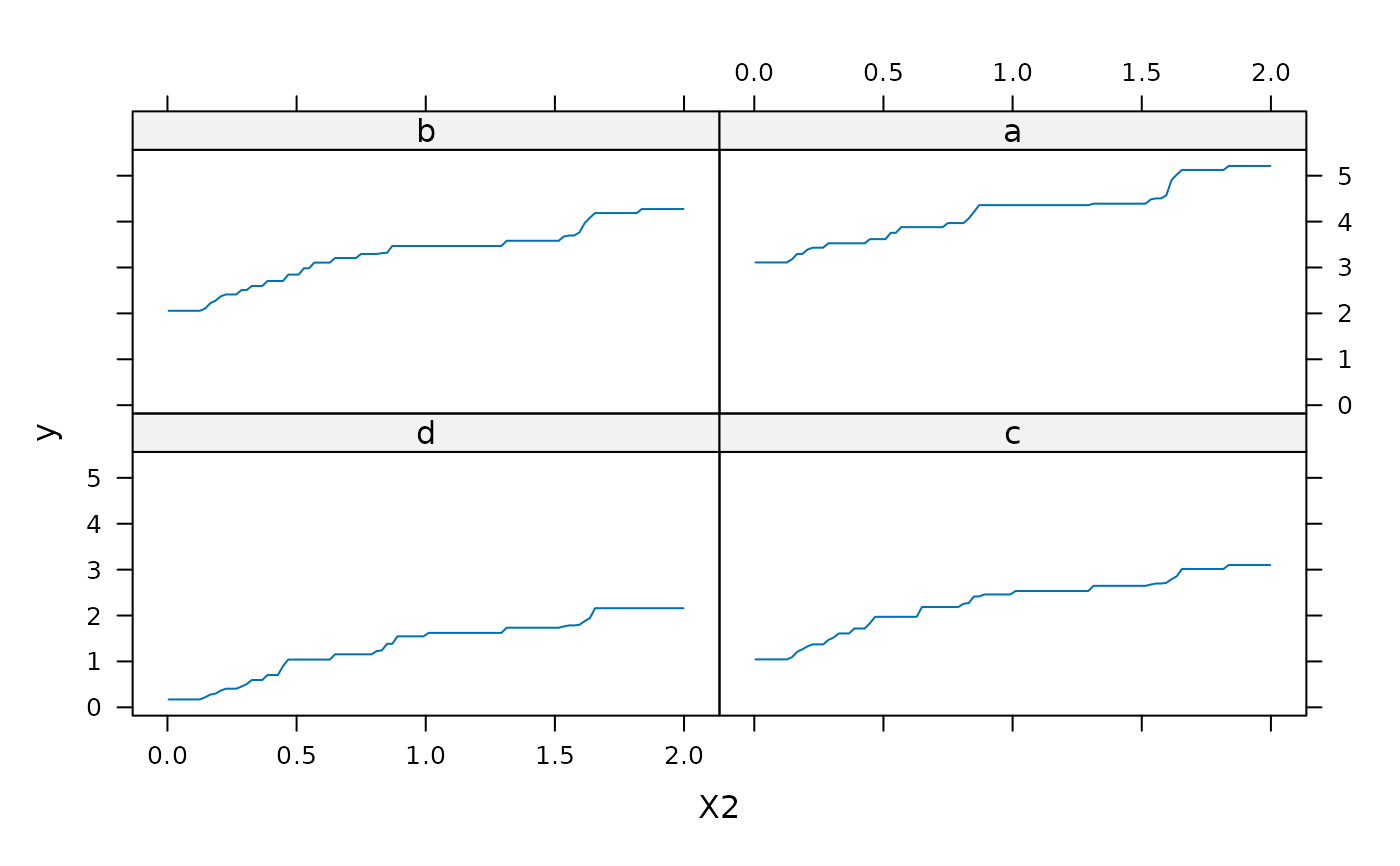
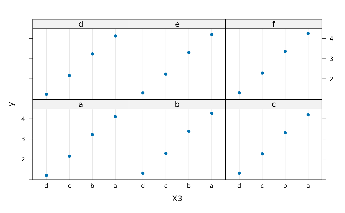
 plot(gbm1, i.var = c("X2", "X3"), n.trees = best.iter)
 plot(gbm1, i.var = 3:4, n.trees = best.iter)
 # Construct trivariate partial dependence plots
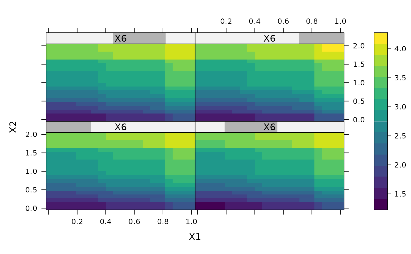
plot(gbm1, i.var = c(1, 2, 6), n.trees = best.iter,
continuous.resolution = 20)
# Construct trivariate partial dependence plots
plot(gbm1, i.var = c(1, 2, 6), n.trees = best.iter,
continuous.resolution = 20)
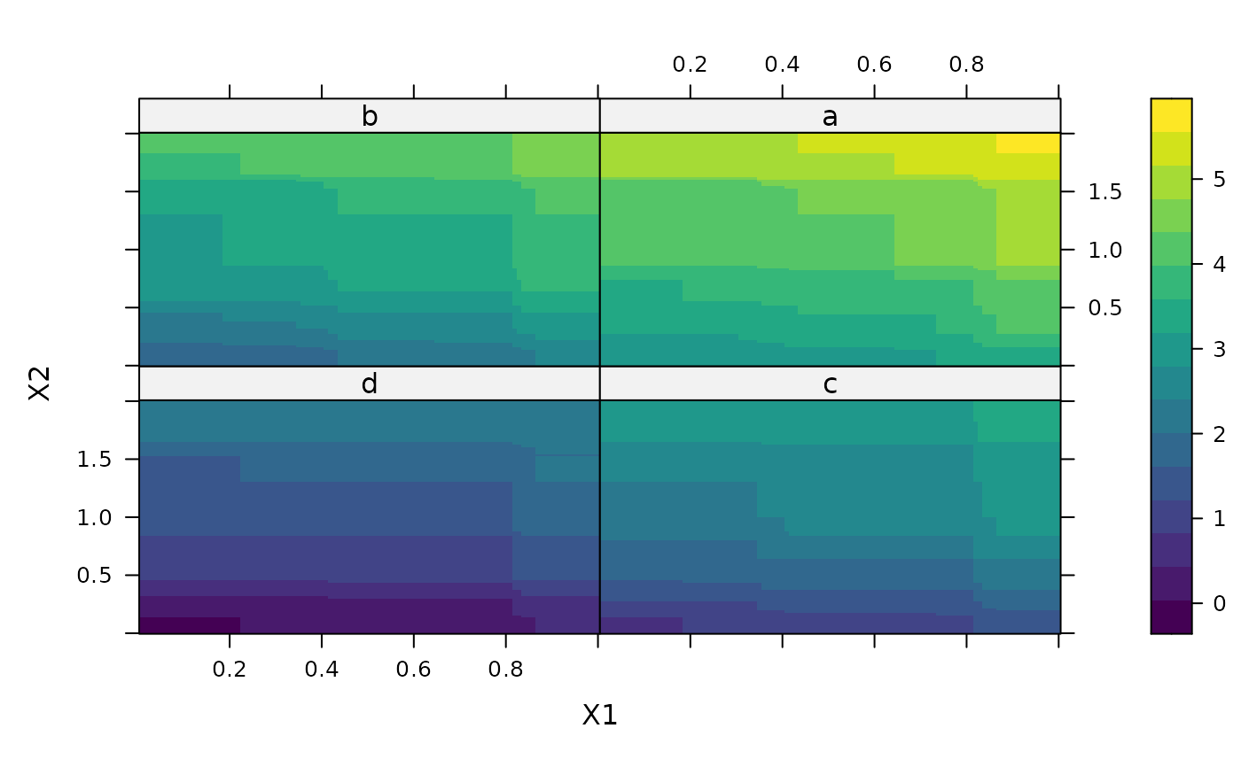
 plot(gbm1, i.var = 1:3, n.trees = best.iter)
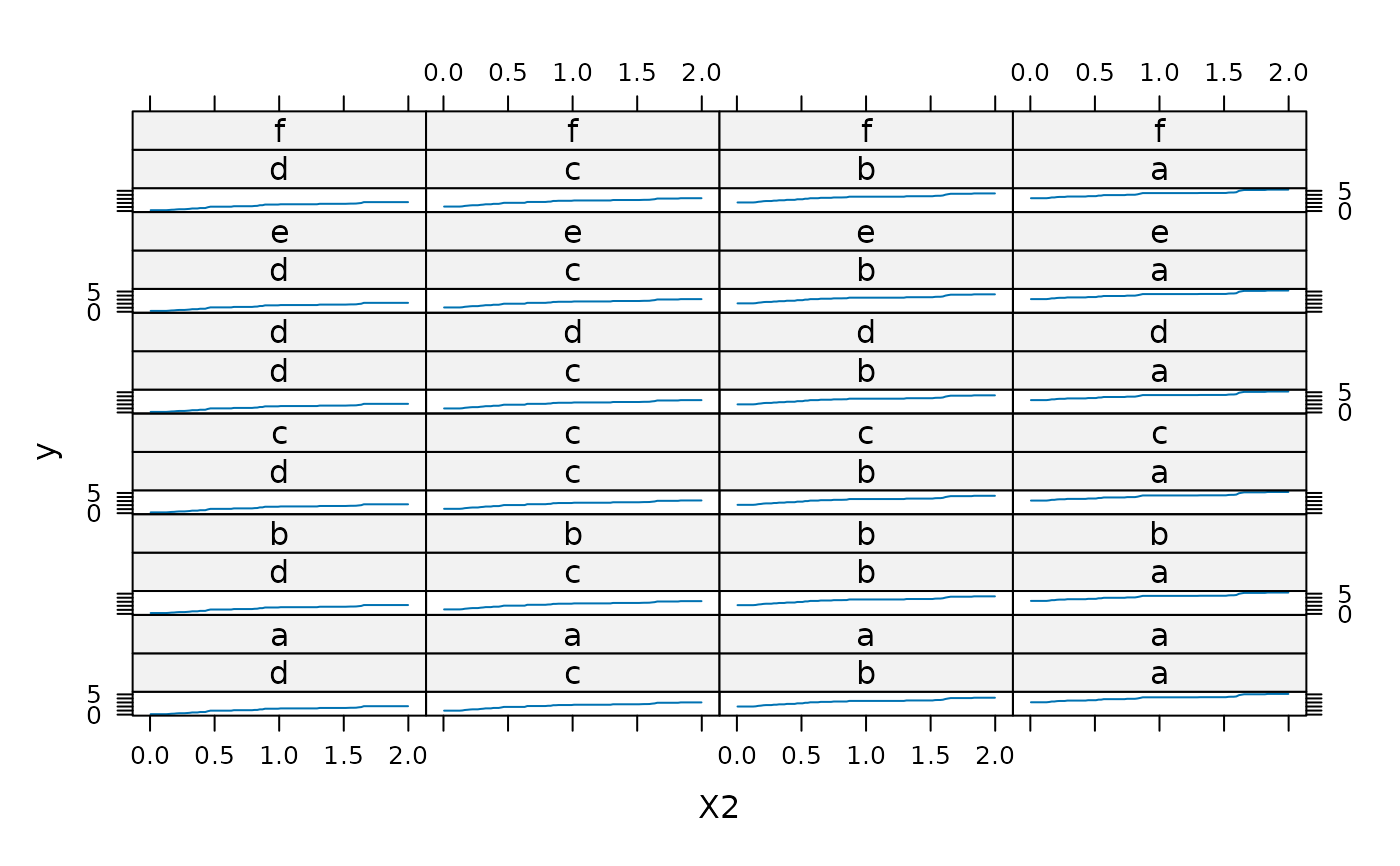
 plot(gbm1, i.var = 2:4, n.trees = best.iter)
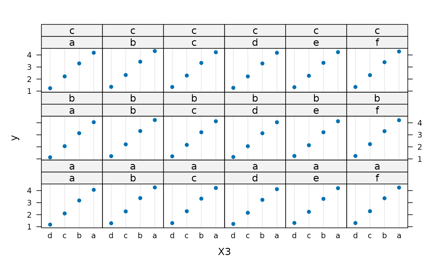
 plot(gbm1, i.var = 3:5, n.trees = best.iter)
 # Add more (i.e., 100) boosting iterations to the ensemble
gbm2 <- gbm.more(gbm1, n.new.trees = 100, verbose = FALSE)
# Add more (i.e., 100) boosting iterations to the ensemble
gbm2 <- gbm.more(gbm1, n.new.trees = 100, verbose = FALSE)