Adds additional trees to a gbm.object object.
Usage
gbm.more(
  object,
  n.new.trees = 100,
  data = NULL,
  weights = NULL,
  offset = NULL,
  verbose = NULL
)
Arguments
- object
A
gbm.objectobject created from an initial call togbm.- n.new.trees
Integer specifying the number of additional trees to add to
object. Default is 100.- data
An optional data frame containing the variables in the model. By default the variables are taken from
environment(formula), typically the environment from whichgbmis called. Ifkeep.data=TRUEin the initial call togbmthengbmstores a copy with the object. Ifkeep.data=FALSEthen subsequent calls togbm.moremust resupply the same dataset. It becomes the user's responsibility to resupply the same data at this point.- weights
An optional vector of weights to be used in the fitting process. Must be positive but do not need to be normalized. If
keep.data=FALSEin the initial call togbmthen it is the user's responsibility to resupply the weights togbm.more.- offset
A vector of offset values.
- verbose
Logical indicating whether or not to print out progress and performance indicators (
TRUE). If this option is left unspecified forgbm.more, then it usesverbosefromobject. Default isFALSE.
Value
A gbm.object object.
Examples
#
# A least squares regression example
#
# Simulate data
set.seed(101) # for reproducibility
N <- 1000
X1 <- runif(N)
X2 <- 2 * runif(N)
X3 <- ordered(sample(letters[1:4], N, replace = TRUE), levels = letters[4:1])
X4 <- factor(sample(letters[1:6], N, replace = TRUE))
X5 <- factor(sample(letters[1:3], N, replace = TRUE))
X6 <- 3 * runif(N)
mu <- c(-1, 0, 1, 2)[as.numeric(X3)]
SNR <- 10 # signal-to-noise ratio
Y <- X1 ^ 1.5 + 2 * (X2 ^ 0.5) + mu
sigma <- sqrt(var(Y) / SNR)
Y <- Y + rnorm(N, 0, sigma)
X1[sample(1:N,size=500)] <- NA # introduce some missing values
X4[sample(1:N,size=300)] <- NA # introduce some missing values
data <- data.frame(Y, X1, X2, X3, X4, X5, X6)
# Fit a GBM
set.seed(102) # for reproducibility
gbm1 <- gbm(Y ~ ., data = data, var.monotone = c(0, 0, 0, 0, 0, 0),
distribution = "gaussian", n.trees = 100, shrinkage = 0.1,
interaction.depth = 3, bag.fraction = 0.5, train.fraction = 0.5,
n.minobsinnode = 10, cv.folds = 5, keep.data = TRUE,
verbose = FALSE, n.cores = 1)
#> CV: 1
#> CV: 2
#> CV: 3
#> CV: 4
#> CV: 5
# Check performance using the out-of-bag (OOB) error; the OOB error typically
# underestimates the optimal number of iterations
best.iter <- gbm.perf(gbm1, method = "OOB")
#> OOB generally underestimates the optimal number of iterations although predictive performance is reasonably competitive. Using cv_folds>1 when calling gbm usually results in improved predictive performance.
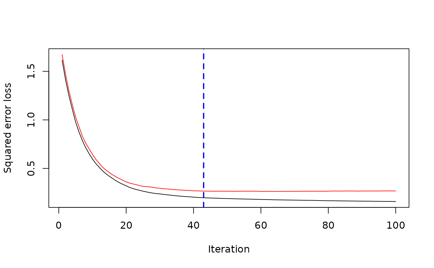 print(best.iter)
#> [1] 43
#> attr(,"smoother")
#> Call:
#> loess(formula = object$oobag.improve ~ x, enp.target = min(max(4,
#> length(x)/10), 50))
#>
#> Number of Observations: 100
#> Equivalent Number of Parameters: 8.32
#> Residual Standard Error: 0.005885
# Check performance using the 50% heldout test set
best.iter <- gbm.perf(gbm1, method = "test")
print(best.iter)
#> [1] 43
#> attr(,"smoother")
#> Call:
#> loess(formula = object$oobag.improve ~ x, enp.target = min(max(4,
#> length(x)/10), 50))
#>
#> Number of Observations: 100
#> Equivalent Number of Parameters: 8.32
#> Residual Standard Error: 0.005885
# Check performance using the 50% heldout test set
best.iter <- gbm.perf(gbm1, method = "test")
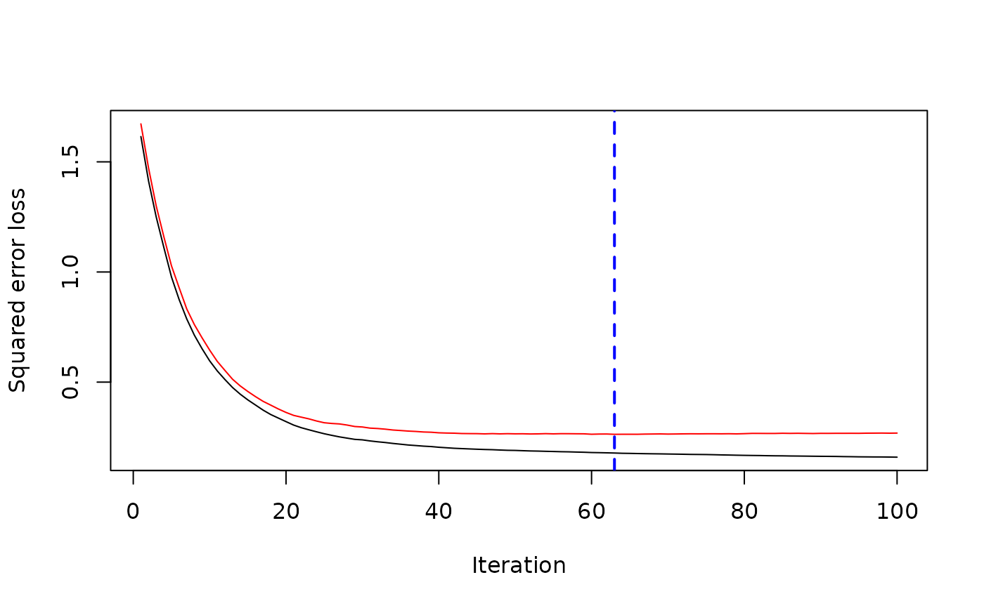 print(best.iter)
#> [1] 63
# Check performance using 5-fold cross-validation
best.iter <- gbm.perf(gbm1, method = "cv")
print(best.iter)
#> [1] 63
# Check performance using 5-fold cross-validation
best.iter <- gbm.perf(gbm1, method = "cv")
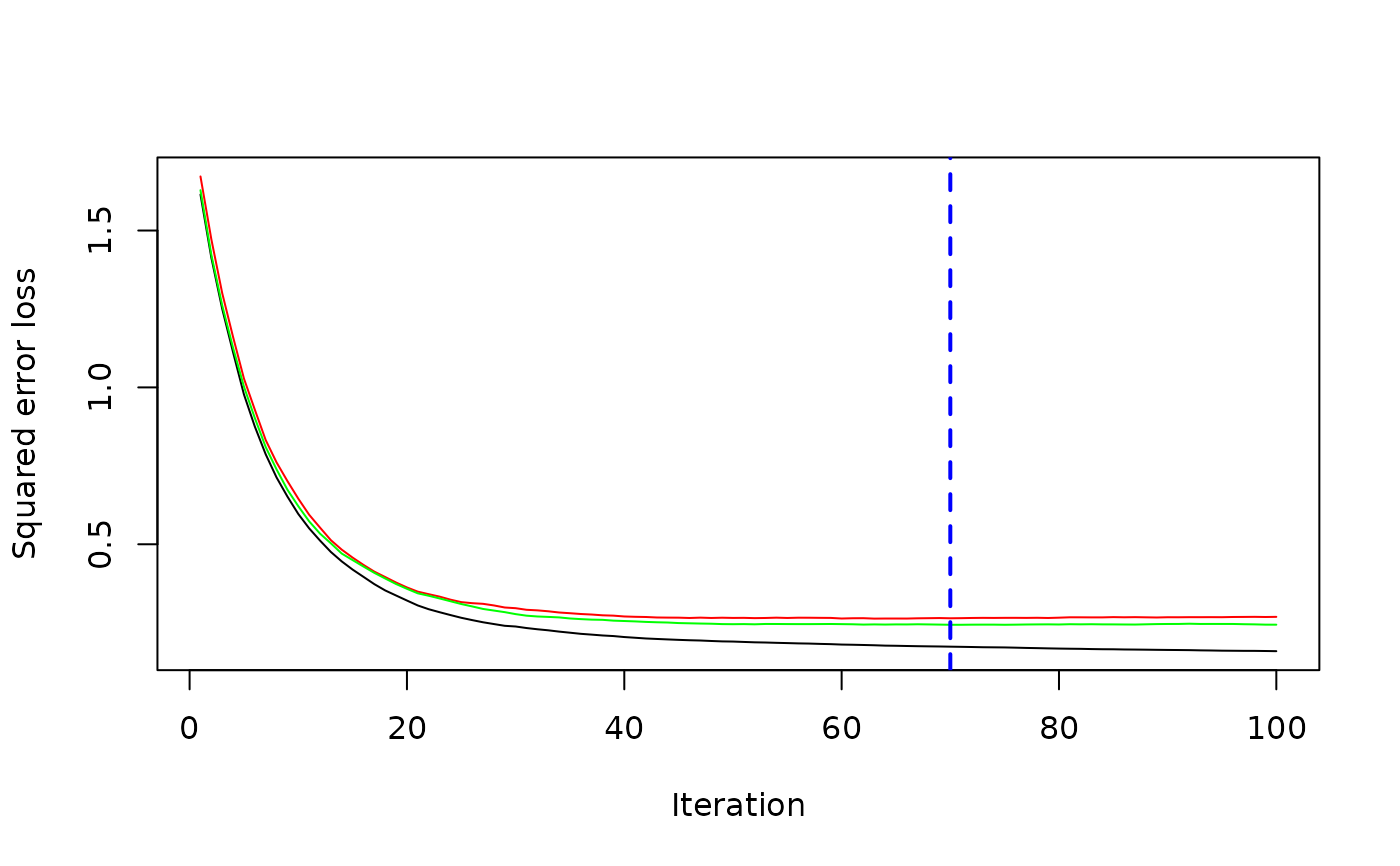 print(best.iter)
#> [1] 70
# Plot relative influence of each variable
par(mfrow = c(1, 2))
summary(gbm1, n.trees = 1) # using first tree
#> var rel.inf
#> X3 X3 86.74183
#> X2 X2 13.25817
#> X1 X1 0.00000
#> X4 X4 0.00000
#> X5 X5 0.00000
#> X6 X6 0.00000
summary(gbm1, n.trees = best.iter) # using estimated best number of trees
print(best.iter)
#> [1] 70
# Plot relative influence of each variable
par(mfrow = c(1, 2))
summary(gbm1, n.trees = 1) # using first tree
#> var rel.inf
#> X3 X3 86.74183
#> X2 X2 13.25817
#> X1 X1 0.00000
#> X4 X4 0.00000
#> X5 X5 0.00000
#> X6 X6 0.00000
summary(gbm1, n.trees = best.iter) # using estimated best number of trees
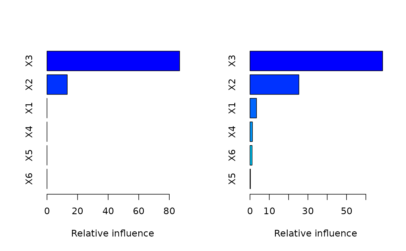 #> var rel.inf
#> X3 X3 68.6902290
#> X2 X2 25.3361275
#> X1 X1 3.3863779
#> X4 X4 1.2681014
#> X6 X6 1.0914539
#> X5 X5 0.2277102
# Compactly print the first and last trees for curiosity
print(pretty.gbm.tree(gbm1, i.tree = 1))
#> SplitVar SplitCodePred LeftNode RightNode MissingNode ErrorReduction Weight
#> 0 2 1.500000000 1 5 9 258.70575 250
#> 1 1 0.643849456 2 3 4 45.93610 122
#> 2 -1 -0.204032200 -1 -1 -1 0.00000 34
#> 3 -1 -0.067172308 -1 -1 -1 0.00000 88
#> 4 -1 -0.105313590 -1 -1 -1 0.00000 122
#> 5 2 2.500000000 6 7 8 41.83219 128
#> 6 -1 0.044497873 -1 -1 -1 0.00000 68
#> 7 -1 0.159057141 -1 -1 -1 0.00000 60
#> 8 -1 0.098197530 -1 -1 -1 0.00000 128
#> 9 -1 -0.001115896 -1 -1 -1 0.00000 250
#> Prediction
#> 0 -0.001115896
#> 1 -0.105313590
#> 2 -0.204032200
#> 3 -0.067172308
#> 4 -0.105313590
#> 5 0.098197530
#> 6 0.044497873
#> 7 0.159057141
#> 8 0.098197530
#> 9 -0.001115896
print(pretty.gbm.tree(gbm1, i.tree = gbm1$n.trees))
#> SplitVar SplitCodePred LeftNode RightNode MissingNode ErrorReduction Weight
#> 0 0 0.582418997 1 2 3 0.9193604 250
#> 1 -1 0.006219724 -1 -1 -1 0.0000000 63
#> 2 -1 -0.010214328 -1 -1 -1 0.0000000 57
#> 3 3 51.000000000 4 8 9 0.7852138 130
#> 4 1 1.016134987 5 6 7 0.5866318 62
#> 5 -1 0.003627100 -1 -1 -1 0.0000000 33
#> 6 -1 -0.015867874 -1 -1 -1 0.0000000 29
#> 7 -1 -0.005491517 -1 -1 -1 0.0000000 62
#> 8 -1 0.010784760 -1 -1 -1 0.0000000 28
#> 9 -1 0.009523251 -1 -1 -1 0.0000000 40
#> Prediction
#> 0 0.0006082206
#> 1 0.0062197235
#> 2 -0.0102143276
#> 3 0.0026340711
#> 4 -0.0054915172
#> 5 0.0036270997
#> 6 -0.0158678743
#> 7 -0.0054915172
#> 8 0.0107847602
#> 9 0.0095232507
# Simulate new data
set.seed(103) # for reproducibility
N <- 1000
X1 <- runif(N)
X2 <- 2 * runif(N)
X3 <- ordered(sample(letters[1:4], N, replace = TRUE))
X4 <- factor(sample(letters[1:6], N, replace = TRUE))
X5 <- factor(sample(letters[1:3], N, replace = TRUE))
X6 <- 3 * runif(N)
mu <- c(-1, 0, 1, 2)[as.numeric(X3)]
Y <- X1 ^ 1.5 + 2 * (X2 ^ 0.5) + mu + rnorm(N, 0, sigma)
data2 <- data.frame(Y, X1, X2, X3, X4, X5, X6)
# Predict on the new data using the "best" number of trees; by default,
# predictions will be on the link scale
Yhat <- predict(gbm1, newdata = data2, n.trees = best.iter, type = "link")
# least squares error
print(sum((data2$Y - Yhat)^2))
#> [1] 5153.285
# Construct univariate partial dependence plots
plot(gbm1, i.var = 1, n.trees = best.iter)
#> var rel.inf
#> X3 X3 68.6902290
#> X2 X2 25.3361275
#> X1 X1 3.3863779
#> X4 X4 1.2681014
#> X6 X6 1.0914539
#> X5 X5 0.2277102
# Compactly print the first and last trees for curiosity
print(pretty.gbm.tree(gbm1, i.tree = 1))
#> SplitVar SplitCodePred LeftNode RightNode MissingNode ErrorReduction Weight
#> 0 2 1.500000000 1 5 9 258.70575 250
#> 1 1 0.643849456 2 3 4 45.93610 122
#> 2 -1 -0.204032200 -1 -1 -1 0.00000 34
#> 3 -1 -0.067172308 -1 -1 -1 0.00000 88
#> 4 -1 -0.105313590 -1 -1 -1 0.00000 122
#> 5 2 2.500000000 6 7 8 41.83219 128
#> 6 -1 0.044497873 -1 -1 -1 0.00000 68
#> 7 -1 0.159057141 -1 -1 -1 0.00000 60
#> 8 -1 0.098197530 -1 -1 -1 0.00000 128
#> 9 -1 -0.001115896 -1 -1 -1 0.00000 250
#> Prediction
#> 0 -0.001115896
#> 1 -0.105313590
#> 2 -0.204032200
#> 3 -0.067172308
#> 4 -0.105313590
#> 5 0.098197530
#> 6 0.044497873
#> 7 0.159057141
#> 8 0.098197530
#> 9 -0.001115896
print(pretty.gbm.tree(gbm1, i.tree = gbm1$n.trees))
#> SplitVar SplitCodePred LeftNode RightNode MissingNode ErrorReduction Weight
#> 0 0 0.582418997 1 2 3 0.9193604 250
#> 1 -1 0.006219724 -1 -1 -1 0.0000000 63
#> 2 -1 -0.010214328 -1 -1 -1 0.0000000 57
#> 3 3 51.000000000 4 8 9 0.7852138 130
#> 4 1 1.016134987 5 6 7 0.5866318 62
#> 5 -1 0.003627100 -1 -1 -1 0.0000000 33
#> 6 -1 -0.015867874 -1 -1 -1 0.0000000 29
#> 7 -1 -0.005491517 -1 -1 -1 0.0000000 62
#> 8 -1 0.010784760 -1 -1 -1 0.0000000 28
#> 9 -1 0.009523251 -1 -1 -1 0.0000000 40
#> Prediction
#> 0 0.0006082206
#> 1 0.0062197235
#> 2 -0.0102143276
#> 3 0.0026340711
#> 4 -0.0054915172
#> 5 0.0036270997
#> 6 -0.0158678743
#> 7 -0.0054915172
#> 8 0.0107847602
#> 9 0.0095232507
# Simulate new data
set.seed(103) # for reproducibility
N <- 1000
X1 <- runif(N)
X2 <- 2 * runif(N)
X3 <- ordered(sample(letters[1:4], N, replace = TRUE))
X4 <- factor(sample(letters[1:6], N, replace = TRUE))
X5 <- factor(sample(letters[1:3], N, replace = TRUE))
X6 <- 3 * runif(N)
mu <- c(-1, 0, 1, 2)[as.numeric(X3)]
Y <- X1 ^ 1.5 + 2 * (X2 ^ 0.5) + mu + rnorm(N, 0, sigma)
data2 <- data.frame(Y, X1, X2, X3, X4, X5, X6)
# Predict on the new data using the "best" number of trees; by default,
# predictions will be on the link scale
Yhat <- predict(gbm1, newdata = data2, n.trees = best.iter, type = "link")
# least squares error
print(sum((data2$Y - Yhat)^2))
#> [1] 5153.285
# Construct univariate partial dependence plots
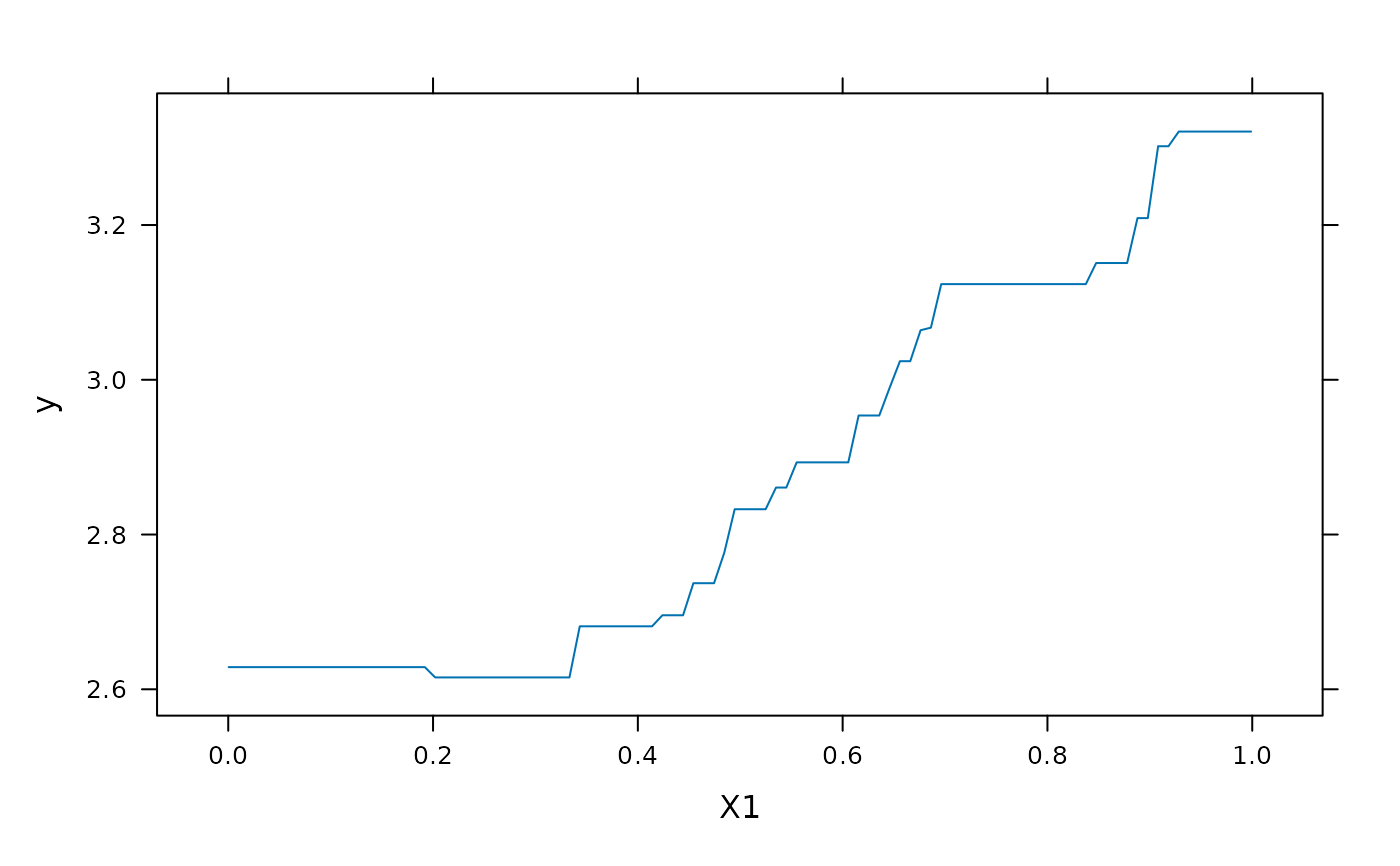
plot(gbm1, i.var = 1, n.trees = best.iter)
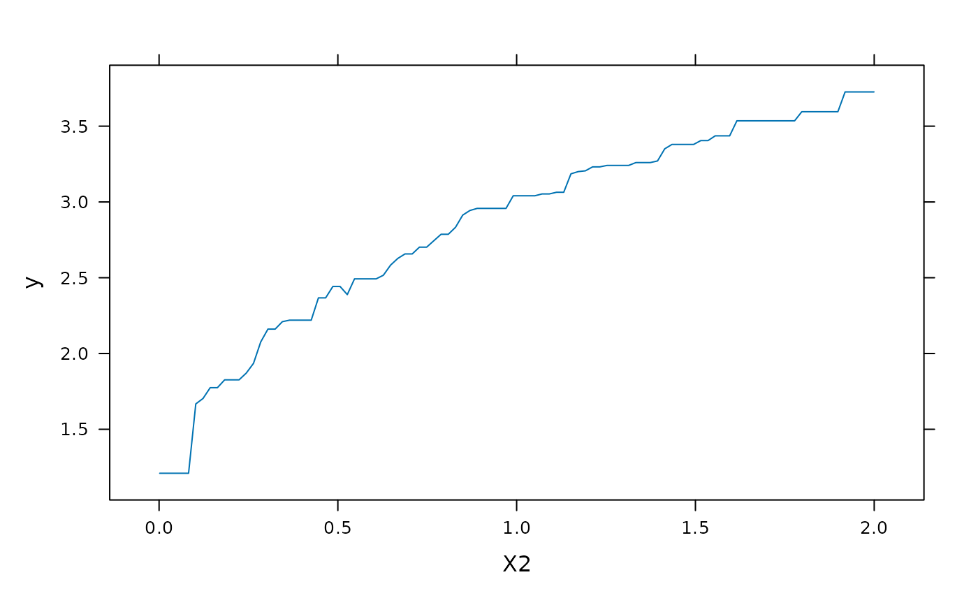
 plot(gbm1, i.var = 2, n.trees = best.iter)
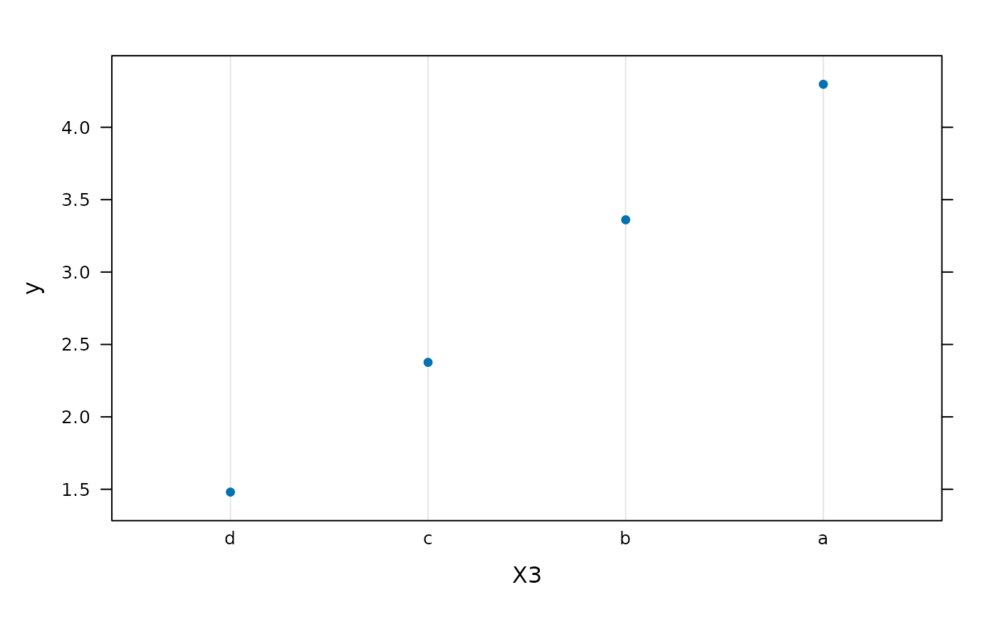
 plot(gbm1, i.var = "X3", n.trees = best.iter) # can use index or name
 # Construct bivariate partial dependence plots
plot(gbm1, i.var = 1:2, n.trees = best.iter)
# Construct bivariate partial dependence plots
plot(gbm1, i.var = 1:2, n.trees = best.iter)
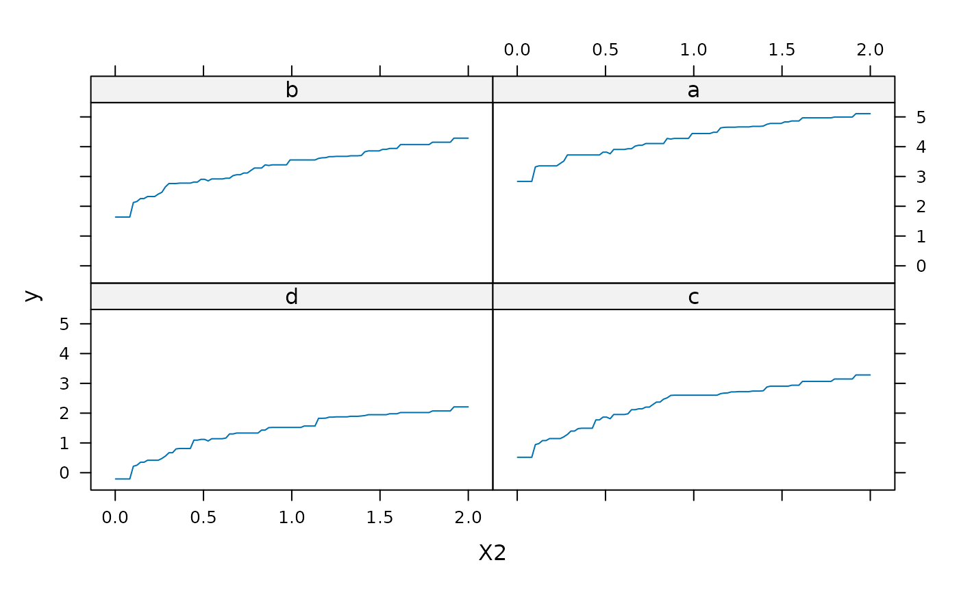
 plot(gbm1, i.var = c("X2", "X3"), n.trees = best.iter)
 plot(gbm1, i.var = 3:4, n.trees = best.iter)
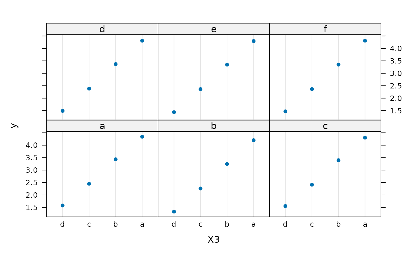 # Construct trivariate partial dependence plots
plot(gbm1, i.var = c(1, 2, 6), n.trees = best.iter,
continuous.resolution = 20)
# Construct trivariate partial dependence plots
plot(gbm1, i.var = c(1, 2, 6), n.trees = best.iter,
continuous.resolution = 20)
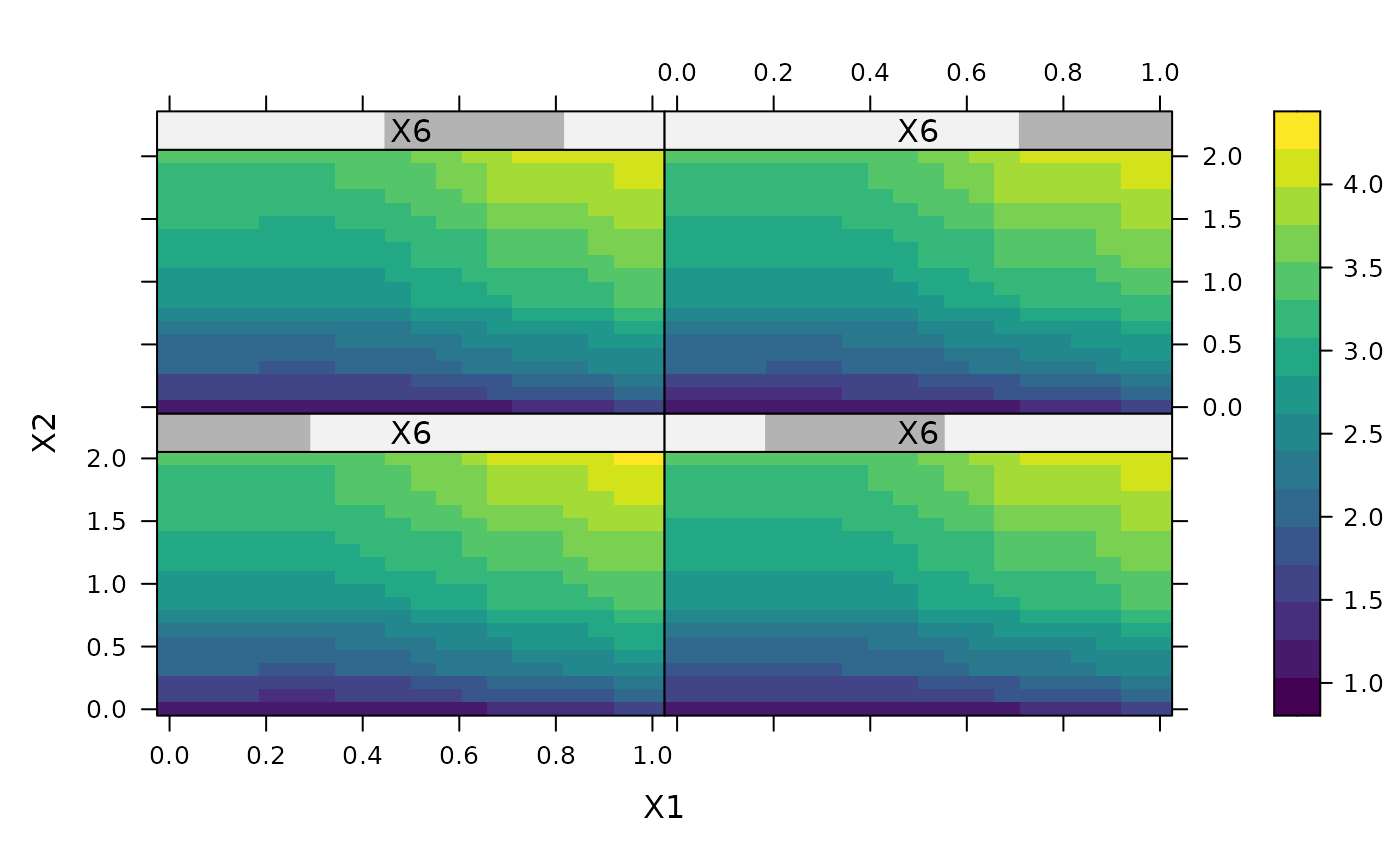 plot(gbm1, i.var = 1:3, n.trees = best.iter)
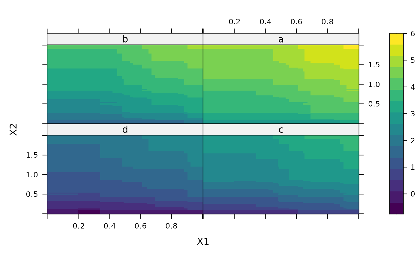 plot(gbm1, i.var = 2:4, n.trees = best.iter)
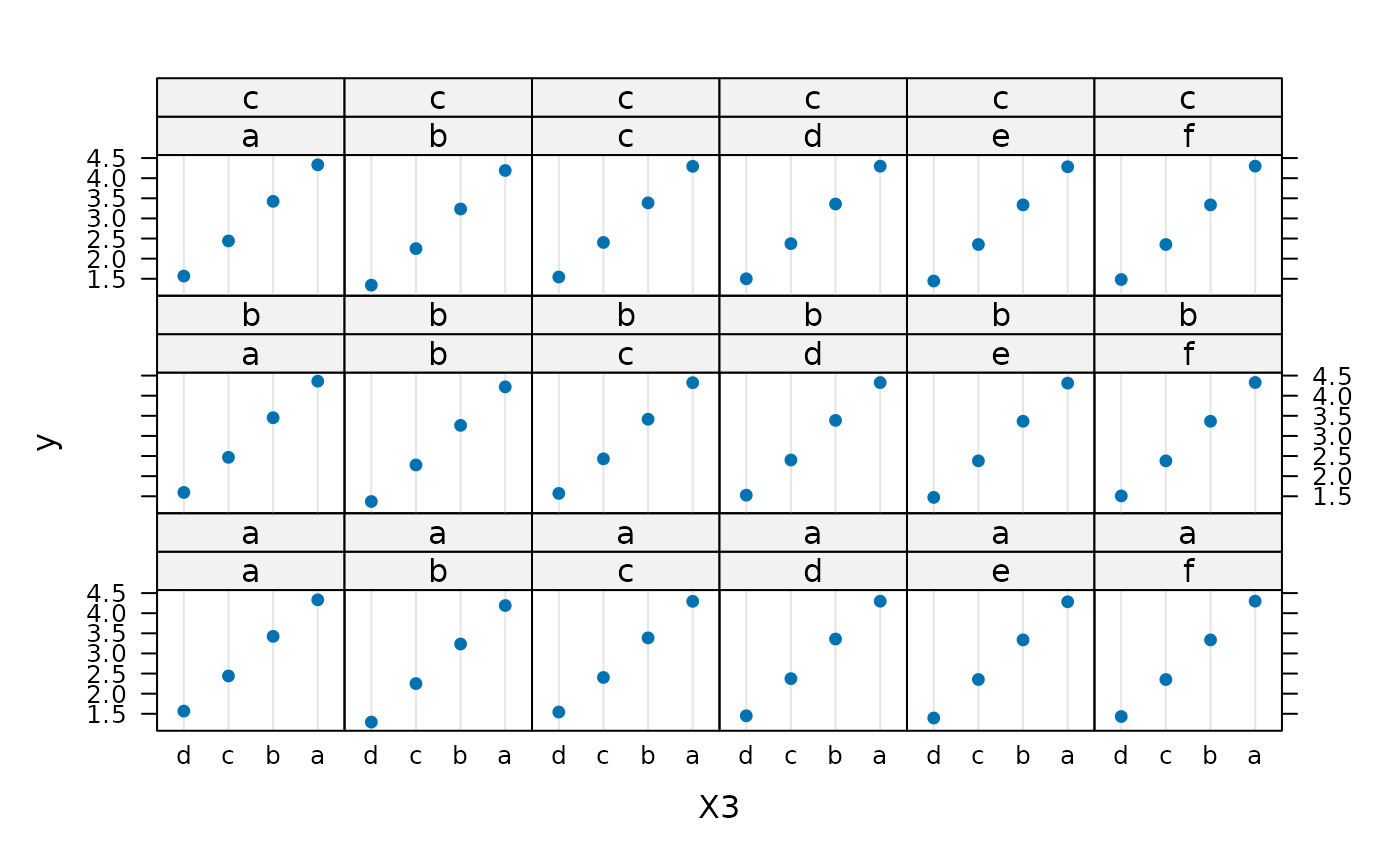
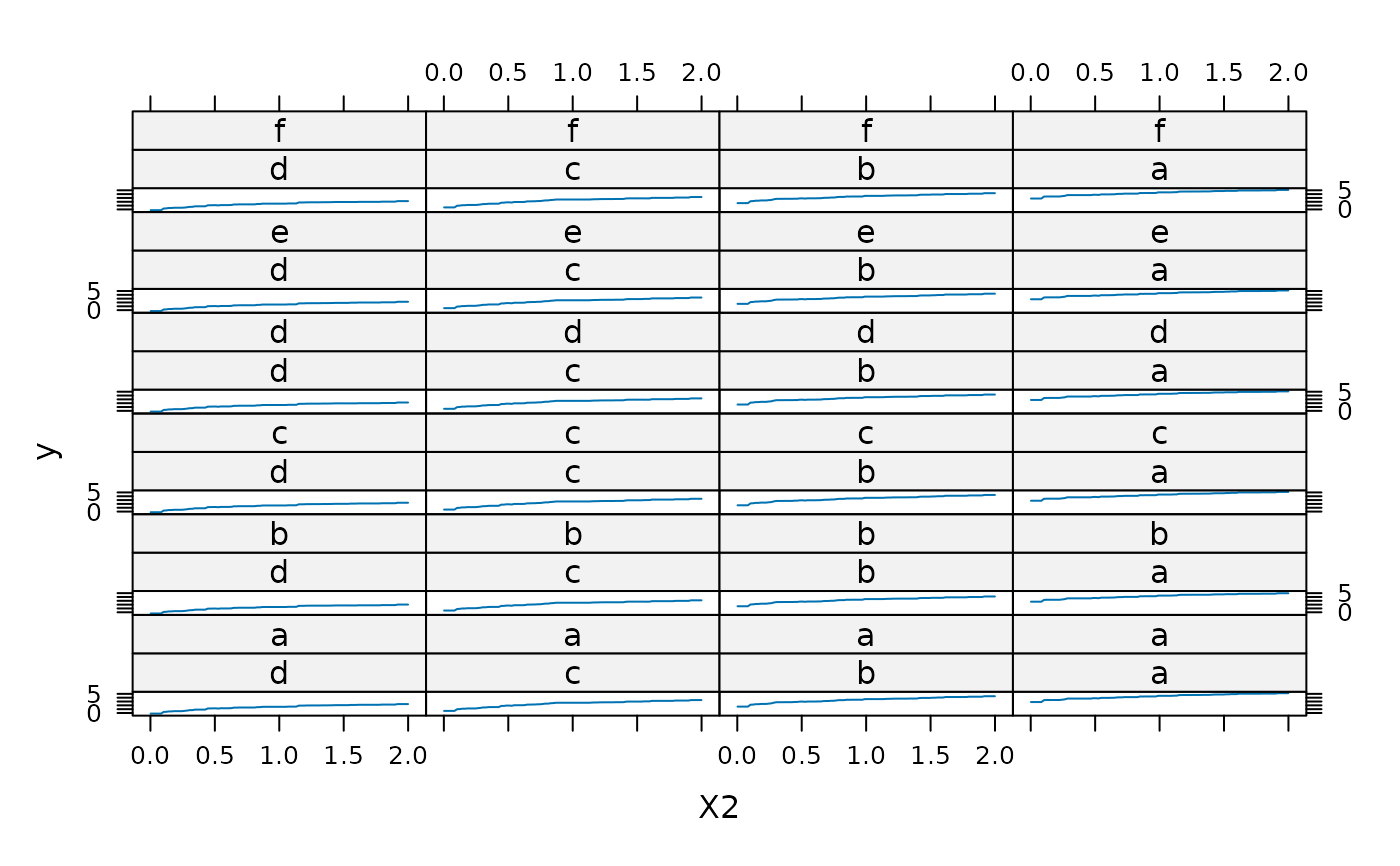 plot(gbm1, i.var = 3:5, n.trees = best.iter)
 # Add more (i.e., 100) boosting iterations to the ensemble
gbm2 <- gbm.more(gbm1, n.new.trees = 100, verbose = FALSE)
# Add more (i.e., 100) boosting iterations to the ensemble
gbm2 <- gbm.more(gbm1, n.new.trees = 100, verbose = FALSE)